fit <- rpart(Kyphosis ~ Age + Number + Start, data = kyphosis)Error in `rpart()`:
! could not find function "rpart"fitError:
! object 'fit' not foundR is different from other tools you may have used.
In Excel, the calculations we carry out in the data are embedded in the spreadsheet containing the data we are working with, in the form of formulas. In contrast, with R, data storage and calculations are generally separated. In some other data analysis tools such as SPSS, we generally point and click on menu options and dialog boxes to allow us to perform statistical analyses. In R, we instead write particular instructions in the form of code. 1
This is because R is a statistical programming language. We write out the particular steps we need to take in one or more scripts - text files containing code. Using a programming language to do data analysis has a number of advantages:
The aim of this worksheet is to introduce you to the basics of R. Nothing will be very complicated - and in fact, the examples are deliberately very simple - but there will be a lot to take in all at once, and it might take you a while to digest everything. The more you work with R, the more these things will become second nature, however. Don’t be afraid to try your own examples in the worksheet below.
Most of the time we will work with R using the desktop application called Rstudio. For the first part of this tutorial, we will use a web interface to R called webr. This will allow us to keep things simple and focus on R itself rather than on the Rstudio interface. The interactive R code boxes (like the one below) allow us to run particular R commands or chunks of code by clicking the Run Code button. You can change or add to what is written in these chunks to address questions given in the workshop, or to experiment and try things out for yourself.
We can also edit the code in the code chunks. Try editing the code above, replacing the + with -, for example.
Try doing some other calculations below.
You can use the standard mathematical symbols. to do this: +, -, /. Note that * is used for multiplication, and ** or ^ to raise something to a power. In R code, these symbols are called operators.
Generally, we want to use the results of one calculation in the next step of our analysis. We therefore store the results of as objects. To create an R object, we first write the name we would like to give the object, followed by an arrow symbol created by the \(<\) and \(-\) symbols next to each other, followed by the thing we want to store.
Note that you can’t have spaces in the names of R objects, as these are used to separate different bits of R code. If you try to do create an object with a space in it, you will get an error message (see below for more on error messages).
R objects come in many different forms, from single numbers to whole datasets, and from chunks of text to the results of regression analysis.
When R objects are simply numbers, we can perform simple calculations with them as we did with the ‘raw’ numbers.
There are several basic types of data in R, from which more complicated data structures are built.
As the name suggests, this type corresponds to numeric data, including decimals (or ‘doubles’). 2. We can create a numeric object in the same way as we did above:
Note that if we just type the name of an object into R, it’s value or other information about it will be printed to screen.
This type corresponds to text data, and we indicate to R that we are working with such data by enclosing the text in quotes "
This type can only ever be one of two values, TRUE or FALSE. Sometimes, you will see these used in abbreviated fashion as T or F.
Functions are pre-existing bits of R code that we can re-use to perform a specific task.
Such tasks include loading a dataset, calculating the data’s descriptive statistics, and running a simple linear regression.
You can also use functions to do simple tasks such as computing a mean or rounding a variable.
function(argument1, argument2, ...)
These arguments could be data stored in R objects, files to open or options controlling the behaviour etc
There may by only one argument or several, and in some cases there may be zero.
For example, if you want to round the number 3.1415 you can use the function round
NB: the real value of \(\pi\) is stored in the pre-existing object pi.
The functions may have more than one argument. The order in which arguments are written determines how they are used by the function. With the round argument, the second argument tells R how many digits to keep after the decimal point when rounding.
The digits argument is optional, so if it is not specified, the default value of 0 is used instead. Instead of using the position of the arguments, we can use the name of the arguments instead. The round functions arguments are named x (the thing to be rounded) and digits.
We can find out the names of the arguments to any particular functions by accessing it’s help file - on which more below.
The basic data types can be combined within data structures. R has several of these.
Vectors are the simplest of the data types, most commonly consisting of sequences of numbers or text. We can create vectors using the c() function, with elements of the vector separated by commas:
You cannot mix data types within a vector, however:
You can also create vectors consisting of a range of integers by writing the start and end of the range you want, separated by a colon:
Sometimes, we want to select particular elements from within a vector. To do this, we write the name of the vector, followed by square brackets, and the position of the thing we want within the vector. This is known as ‘indexing’.
For instance, if we want the second element from the list of cat names, we write:
We can select more than one element using ‘slicing’. We use the same range method as before:
You can find the length of a vector using the length function.
}}
To find our more information about a particular function, we can use the help function. For instance, to find out more about the mean function, we can call the help function with mean as the argument:
This is usually instantaneous, but takes a few seconds in the web version of R.
Try to calculate the mean of the first 5 numbers of the my_numbers vector we created above.
You may have noticed in the help file for the mean function, there is an argument to the function called na.rm. This stands for ‘NA remove’. NA stands for ‘Not Available’, and is used by R to represent missing values. If we try to calculate the mean of a vector containing missing values, we will obtain a missing value. This is to ensure that we always know when we might have a problem with our calculations due to missing or invalid data.
seq is doing in the code above? Try using the seq function in the space below, and use the help function to find out how it works. Some of the help file may be confusing, but focus on the bits under the argument heading Arguments and Value.na.rm argument to the mean function as T, and also via indexing.Lists are very similar to vectors, but can include data of different types. This means calculations with them are a bit slower, but they are more flexible. You can also provide a name for each entry within the list. We create lists using the list function:
We can extract specific elements from a list using the $ symbol:
We can also index elements, but to extract them we should use the double square brackets:
These are probably the data structure in R you will use most often. They are used for holding whole datasets. Practically speaking, they are lists of vectors of equal length.
The built-in dataset iris is a good example of a dataframe. We can look at the first few rows of this dataframe using the head function:
As with lists, we can access particular columns using the $ symbol.
As with vectors, we can slice away particular parts of the dataframe. In this case we select the 10th to the 20th row, and the second and third column.
We can also do this by name:
Check you understand what the above code is doing, using the help function if necessary.
A matrix is another collection of vectors, but is somewhat simpler than a dataframe. All elements of a matrix must have the same type, and column names are not required. We create a matrix using the matrix function ( surprise surprise), often from vectors.
Logical data results whenever we use conditions. For instance, we might check if value of variable is greater than a particular number, using the greater than > operator.
We can also use the <, >= and <= operators to check for “less than”, “greater than or equal to”, or “less than or equal to” relationships.
To test whether to values are equal, we can use the ==, which means “is equal to”. Note that we must use two = symbols, otherwise our code will not work.
These logical conditions are important when writing R code, because it allows our R scripts to do different things depending on what inputs are given to it.
We do this using if / else clauses:
If the condition beside the if statement is true, the first print statement is executed (run). Otherwise, the part in the else clause is run (the bit enclosed in else{…}).
When we do something wrong, R will give us an error message. At first, these can seem quite mysterious. It is important to read error messages, however, because they often help you understand what you have done wrong.
Subscript out of bounds. This means that you have tried to go beyond the end of a vector, list or dataframe. For example, you have tried to access the 10th number in a list that is only 9 numbers long. You can find out how long a list is by using the function length. Similarly, the function dim (for ‘dimension’) tells you the number of rows and columns in a dataframe.non-numeric argument to binary operator. This sounds like gibberish, but generally it just means your data is of the wrong type. An operator in R represents a mathematical calculation like +, -, *, or /. If we try to use these, for instance, text data, we get this error.Run the code below, and see if you can work out how to fix it.
Often this can happen when you read in data that has a mix of numeric an character data in one of the columns.
object "unicorn" was not found. This error occurs when you try to access an R object (unicorn in this case) that doesn’t exist. This could be because you have typed the name wrong, or because you are running your code in the wrong order and you haven’t created it yet.See the example below and try to fix it.
Could not find function "help_me". Similarly, this happens when you try to use a function that doesn’t exist. This might be because of a mis-typing 3. See the example below.Object of type 'closure' is not subsettable Another strange-sounding message. This occurs when you try to use indexing on a function:Often, we want to repeat the same chunk of code many times. For-loops are one way of doing this. These take values from a vector or list one at a time, and storing each value in iteration in an iteration variable, often called i.
If we wanted to add two vectors together, we could do this using a for loop:
However, R has built in ways of dealing with simple operations on vectors. Mathematical operations on vectors in R are automatically vectorised - the first elements of each vector are added together and stored in first element of the answer object, and the same happens with each subsequent position:
Not everything can be easily vectorised, however, and for particularly complex calculations, it may be necessary to write for loops.
Rstudio is a good way to work with R.
Rstudio and you should see the rstudio icon appear![]()
From this point, you should work with Rstudio rather than with webR.
When you open Rstudio, you will see something that looks like the image below.
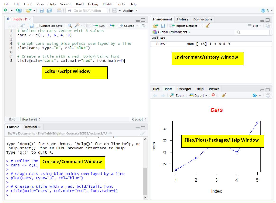
The different bits of the Rstudio window have been labelled in yellow in the image, and are explained in more detail below.
The console/command window is where you can type commands. Type the command next to the \(>\) sign and press ENTER
The editor/script window is where you can edit and save commands. To run commands from here highlight the command and either click Run or type CTRL+ENTER. This will run the line your cursor is currently on, or the code you have highlighted (which could be multiple lines).
The environment pane of the environment/history window shows the data you have loaded and any values your have created during your session. You can have a closer look by clicking on them. The history pane shows a history of your typed commands
The files/plots/packages/help window has panes that allow you to open files, view plots, install and load packages, or use the help function
To be able to work effectively we will create “RStudio projects” which is a feature of RStudio that allows us to keep the data, code and outputs for one project in one folder.
This organizes our work, helps us prevent mistakes when loading and saving files, and makes it easier to switch between different projects.
Within a project, group together all code relating to a particular step in a separate scripts. A script is just a file containing R code.
Scripts can be saved in the project folder (you might like to create a folder called scripts within your folder), and they can be revisited and amended
By adding comments in our scripts, we can add notes explaining what each command is meant to do. This might help others understand our thought process, or even the Future You who revisits your code at a later date!
To create a new project in RStudio:
To open an “existing project” in RStudio, go to the project folder (directory) and double click on the .Rproj file in that directory.
Alternatively, you can use the open project dialog in the menu on the top right of the Rstudio screen.
Once you create an RStudio Project, then you should create a Script. To create a Script:
Packages are collections of R code designed to perform specific tasks. These may be included in R by default, or they may be written by other R users. R has a vibrant community of statisticians, data scientists, biologists, epidemiologists, economists, geographers, etc. etc. who contribute code relating to their discipline.
To use functions from a package, we first need to load it from our package library using the library function.
For instance, we can load in the rpart package for tree-based models (on which more later in the course). This package is included in the base R installation.
Don’t worry about what the code is doing for the moment, just notice that if we try to use a function from the rpart package without first loading the package we get an error:
fit <- rpart(Kyphosis ~ Age + Number + Start, data = kyphosis)Error in `rpart()`:
! could not find function "rpart"fitError:
! object 'fit' not foundlibrary(rpart)
fit <- rpart(Kyphosis ~ Age + Number + Start, data = kyphosis)
fitn= 81
node), split, n, loss, yval, (yprob)
* denotes terminal node
1) root 81 17 absent (0.79012346 0.20987654)
2) Start>=8.5 62 6 absent (0.90322581 0.09677419)
4) Start>=14.5 29 0 absent (1.00000000 0.00000000) *
5) Start< 14.5 33 6 absent (0.81818182 0.18181818)
10) Age< 55 12 0 absent (1.00000000 0.00000000) *
11) Age>=55 21 6 absent (0.71428571 0.28571429)
22) Age>=111 14 2 absent (0.85714286 0.14285714) *
23) Age< 111 7 3 present (0.42857143 0.57142857) *
3) Start< 8.5 19 8 present (0.42105263 0.57894737) *Most packages do not come pre-installed. We install them using the install.packages function. Try running the code below in Rstudio:
install.packages("tibble")Unlike when you are using the library() function, you must enclose the name of the package you wish to install in quotes, or else you will get an error. The tibble package provide easier-to-read dataframes, along with additional special features.
library(tibble)

as_tibble(iris)
# A tibble: 150 × 5
Sepal.Length Sepal.Width Petal.Length Petal.Width Species
<dbl> <dbl> <dbl> <dbl> <fct>
1 5.1 3.5 1.4 0.2 setosa
2 4.9 3 1.4 0.2 setosa
3 4.7 3.2 1.3 0.2 setosa
4 4.6 3.1 1.5 0.2 setosa
5 5 3.6 1.4 0.2 setosa
6 5.4 3.9 1.7 0.4 setosa
7 4.6 3.4 1.4 0.3 setosa
8 5 3.4 1.5 0.2 setosa
9 4.4 2.9 1.4 0.2 setosa
10 4.9 3.1 1.5 0.1 setosa
# ℹ 140 more rowsNote that you only need to install a package once on each machine that you are using 4
Housekeeping tip! When you write a script, begin by loading all your packages at the very top of the script.
If you want to open an .xls (excel) file in RStudio follow these steps:
readxl as discussed above.readxl:install.packages("readxl")library(readxl)my_data <- read_excel("data/wage2.xls")In this example, we named the object “mydata”. You can now see this object in the top-right Environment window.
head(my_data)# A tibble: 6 × 16
wage hours IQ KWW educ exper tenure age married south urban sibs
<dbl> <dbl> <dbl> <dbl> <dbl> <dbl> <dbl> <dbl> <dbl> <dbl> <dbl> <dbl>
1 769 40 93 35 12 11 2 31 1 0 1 1
2 825 40 108 46 14 11 9 33 1 0 1 1
3 650 40 96 32 12 13 7 32 1 0 1 4
4 562 40 74 27 11 14 5 34 1 0 1 10
5 600 40 91 24 10 13 0 30 0 0 1 1
6 1154 45 111 37 15 13 1 36 1 0 0 2
# ℹ 4 more variables: brthord <dbl>, meduc <dbl>, feduc <dbl>, lwage <dbl>summary(my_data) wage hours IQ KWW
Min. : 115.0 Min. :25.00 Min. : 54.0 Min. :13.00
1st Qu.: 699.0 1st Qu.:40.00 1st Qu.: 94.0 1st Qu.:32.00
Median : 937.0 Median :40.00 Median :104.0 Median :37.00
Mean : 988.5 Mean :44.06 Mean :102.5 Mean :36.19
3rd Qu.:1200.0 3rd Qu.:48.00 3rd Qu.:113.0 3rd Qu.:41.00
Max. :3078.0 Max. :80.00 Max. :145.0 Max. :56.00
educ exper tenure age
Min. : 9.00 Min. : 1.0 Min. : 0.000 Min. :28.00
1st Qu.:12.00 1st Qu.: 8.0 1st Qu.: 3.000 1st Qu.:30.00
Median :13.00 Median :11.0 Median : 7.000 Median :33.00
Mean :13.68 Mean :11.4 Mean : 7.217 Mean :32.98
3rd Qu.:16.00 3rd Qu.:15.0 3rd Qu.:11.000 3rd Qu.:36.00
Max. :18.00 Max. :22.0 Max. :22.000 Max. :38.00
married south urban sibs
Min. :0.0000 Min. :0.0000 Min. :0.0000 Min. : 0.000
1st Qu.:1.0000 1st Qu.:0.0000 1st Qu.:0.0000 1st Qu.: 1.000
Median :1.0000 Median :0.0000 Median :1.0000 Median : 2.000
Mean :0.9005 Mean :0.3228 Mean :0.7195 Mean : 2.846
3rd Qu.:1.0000 3rd Qu.:1.0000 3rd Qu.:1.0000 3rd Qu.: 4.000
Max. :1.0000 Max. :1.0000 Max. :1.0000 Max. :14.000
brthord meduc feduc lwage
Min. : 1.000 Min. : 0.00 Min. : 0.00 Min. :4.745
1st Qu.: 1.000 1st Qu.: 9.00 1st Qu.: 8.00 1st Qu.:6.550
Median : 2.000 Median :12.00 Median :11.00 Median :6.843
Mean : 2.178 Mean :10.83 Mean :10.27 Mean :6.814
3rd Qu.: 3.000 3rd Qu.:12.00 3rd Qu.:12.00 3rd Qu.:7.090
Max. :10.000 Max. :18.00 Max. :18.00 Max. :8.032 Some logical operators that you should know are the following:
& means AND, it returns TRUE if the conditions on both sides of the & are TRUE
| means OR, it returns TRUE when at least of the two sides are TRUE
! means NOT, it returns FALSE if the logical variable is TRUE
== means EQUALS, it is used when specifying a value of an existing variable in and if statement
To access a variable in a dataframe, use $ after the name of the dataframe
#The function `head` will only let us see the first few values
head(my_data$age)
[1] 31 33 32 34 30 36$ to name it and ifelse arguments to specify its values with respect to other variables in the dataframemy_data$age_dummy <- ifelse(my_data$age < 35, "young", "old")
table(my_data$age_dummy)
  old young
231 432 cut function to specify its values with respect to other variables in the dataframemy_data$age_group <- cut(my_data$age, c(27, 30,34, 38))
table(my_data$age_group)
(27,30] (30,34] (34,38]
186 246 231 mydata in the example above), you can estimate some basic by typing the following command:summary(my_data) wage hours IQ KWW
Min. : 115.0 Min. :25.00 Min. : 54.0 Min. :13.00
1st Qu.: 699.0 1st Qu.:40.00 1st Qu.: 94.0 1st Qu.:32.00
Median : 937.0 Median :40.00 Median :104.0 Median :37.00
Mean : 988.5 Mean :44.06 Mean :102.5 Mean :36.19
3rd Qu.:1200.0 3rd Qu.:48.00 3rd Qu.:113.0 3rd Qu.:41.00
Max. :3078.0 Max. :80.00 Max. :145.0 Max. :56.00
educ exper tenure age
Min. : 9.00 Min. : 1.0 Min. : 0.000 Min. :28.00
1st Qu.:12.00 1st Qu.: 8.0 1st Qu.: 3.000 1st Qu.:30.00
Median :13.00 Median :11.0 Median : 7.000 Median :33.00
Mean :13.68 Mean :11.4 Mean : 7.217 Mean :32.98
3rd Qu.:16.00 3rd Qu.:15.0 3rd Qu.:11.000 3rd Qu.:36.00
Max. :18.00 Max. :22.0 Max. :22.000 Max. :38.00
married south urban sibs
Min. :0.0000 Min. :0.0000 Min. :0.0000 Min. : 0.000
1st Qu.:1.0000 1st Qu.:0.0000 1st Qu.:0.0000 1st Qu.: 1.000
Median :1.0000 Median :0.0000 Median :1.0000 Median : 2.000
Mean :0.9005 Mean :0.3228 Mean :0.7195 Mean : 2.846
3rd Qu.:1.0000 3rd Qu.:1.0000 3rd Qu.:1.0000 3rd Qu.: 4.000
Max. :1.0000 Max. :1.0000 Max. :1.0000 Max. :14.000
brthord meduc feduc lwage
Min. : 1.000 Min. : 0.00 Min. : 0.00 Min. :4.745
1st Qu.: 1.000 1st Qu.: 9.00 1st Qu.: 8.00 1st Qu.:6.550
Median : 2.000 Median :12.00 Median :11.00 Median :6.843
Mean : 2.178 Mean :10.83 Mean :10.27 Mean :6.814
3rd Qu.: 3.000 3rd Qu.:12.00 3rd Qu.:12.00 3rd Qu.:7.090
Max. :10.000 Max. :18.00 Max. :18.00 Max. :8.032
age_dummy age_group
Length:663 (27,30]:186
Class :character (30,34]:246
Mode :character (34,38]:231
regression <- lm(dependent ~ independent1 + independent2, data=my_data)where “regression” is the name of the object that contains the regression results, “dependent” is the name of the dependent variable (\(y\)) in the data, and “independent1” and “independent2” are the names of the independent variables (\(x\)) in the data.
After the comma we tell R which dataframe to use to run this regression
Once we run the regression, we need to run another command to display the results:
summary(regression) where “summary” is the function that calls the results of the regression, and “regression” is the name I chose for the object that contains the regression results
TASK: Try running a linear regression model using the wage2.xls data.
It is possible to write SPSS code (called syntax) to carry out particular statistical analyses. Similarly, it is possible to write code to perform particular tasks in excel (called ‘Macros’, using a language called Visual Basic). However, while useful, these alternatives have a narrower array of features and tools available.↩︎
Technically, the numeric type includes both ‘double’ (decimal or real) and ‘integer’ data types. But most of the time you won’t need to worry about this. It is also possible to store complex numbers, which have their own type (but again, don’t worry if this doesn’t mean anything to you).↩︎
Alternatively, it could be because you are trying to use a function from a package that isn’t loaded yet. See the section on packages.↩︎
New versions of R packages are frequently released, so you will need to update the version you have installed sometimes.↩︎